Binomial Distribution
The binomial distribution models the number of successes in a fixed number of independent trials, each with the same probability of success. It is one of the most used distributions in statistics, appearing in quality control, clinical trials, A/B testing, and survey analysis.
Definition
A random variable \(X\) follows a binomial distribution with parameters \(n\) (number of trials) and \(p\) (probability of success per trial), written \(X \sim \text{Binomial}(n, p)\), if:
\[P(X = k) = \binom{n}{k} p^k (1-p)^{n-k}, \quad k = 0, 1, \ldots, n\]
where \(\binom{n}{k} = \frac{n!}{k!(n-k)!}\) is the binomial coefficient, counting the number of ways to arrange \(k\) successes among \(n\) trials.
The binomial distribution has two requirements: the trials must be independent, and the probability of success \(p\) must be constant across all trials. When these hold, \(X\) counts how many of the \(n\) trials result in success.
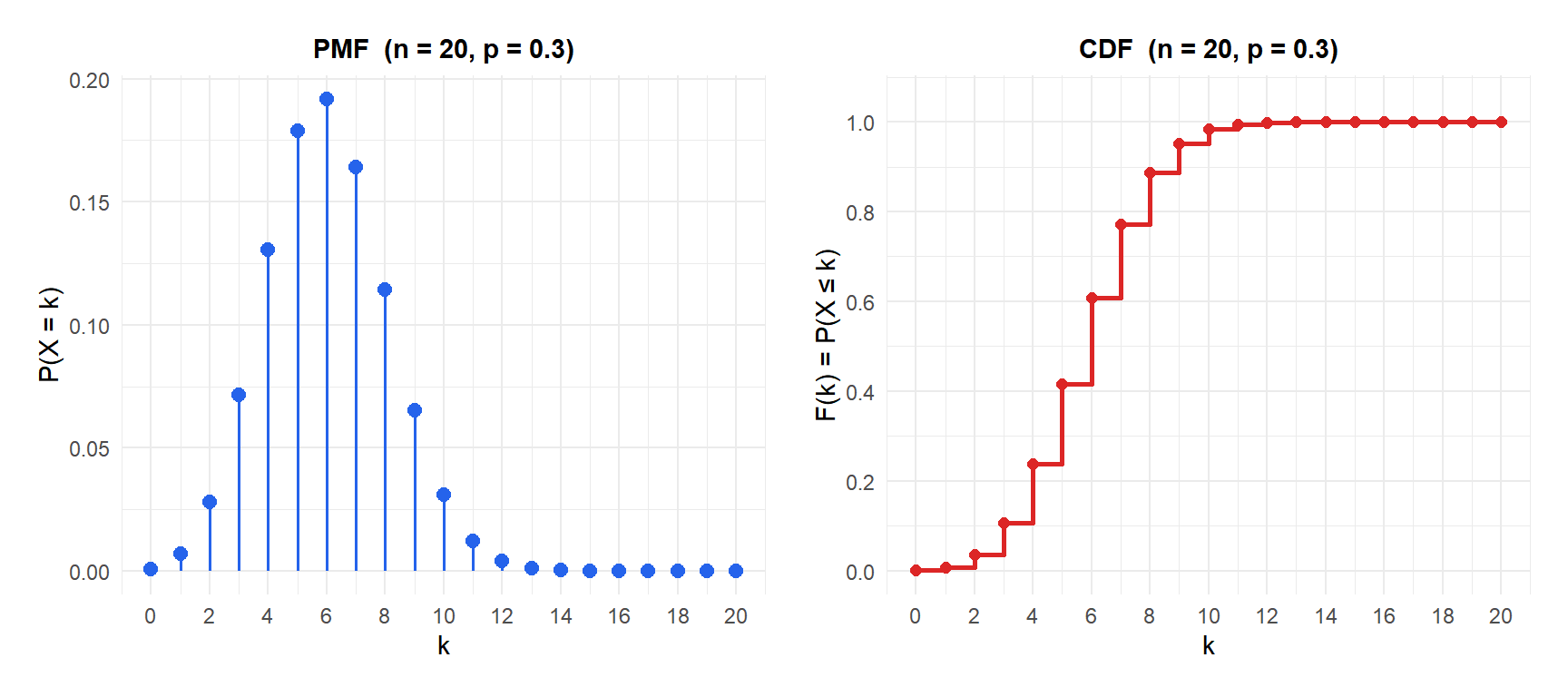
Probability Mass Function and CDF
The PMF gives the probability of exactly \(k\) successes. The cumulative distribution function accumulates these probabilities:
\[F(k) = P(X \leq k) = \sum_{i=0}^{k} \binom{n}{i} p^i (1-p)^{n-i}\]
Properties
For \(X \sim \text{Binomial}(n, p)\):
- Expected Value (Mean)
\[E(X) = np\]
- Variance
\[\text{Var}(X) = np(1-p)\]
- Skewness
\[\text{Skewness} = \frac{1 - 2p}{\sqrt{np(1-p)}}\]
The distribution is symmetric when \(p = 0.5\), right-skewed when \(p < 0.5\), and left-skewed when \(p > 0.5\). As \(n\) increases, the distribution becomes more symmetric regardless of \(p\).
- Kurtosis
\[g_2 = \frac{1 - 6p(1-p)}{np(1-p)}\]
- Quantile Function
The quantile function \(Q(u)\) gives the smallest integer \(k\) such that \(F(k) \geq u\). There is no closed-form expression; it is computed numerically by most software.
Step-by-step example
A pharmaceutical company runs a clinical trial on 15 patients. Based on prior data, the drug has a 40% response rate (\(p = 0.4\)). Let \(X\) = number of patients who respond, \(X \sim \text{Binomial}(15, 0.4)\).
Probability of exactly 6 responses:
\[P(X = 6) = \binom{15}{6}(0.4)^6(0.6)^9 = 5005 \times 0.004096 \times 0.010078 \approx 0.207\]
Expected number of responses:
\[E(X) = 15 \times 0.4 = 6 \text{ patients}\]
Variance and standard deviation:
\[\text{Var}(X) = 15 \times 0.4 \times 0.6 = 3.6, \qquad \text{SD}(X) = \sqrt{3.6} \approx 1.90\]
Probability of 8 or more responses (unusually good result):
\[P(X \geq 8) = 1 - P(X \leq 7) = 1 - F(7) \approx 1 - 0.787 = 0.213\]
About 21% of trials of this size would show 8 or more responders by chance alone.
- A/B testing: 500 users see a new website design, each clicking (success) with probability 0.12. \(X \sim \text{Binomial}(500, 0.12)\). Expected clicks: 60.
- Quality control: a batch of 200 components has a 2% defect rate. \(X \sim \text{Binomial}(200, 0.02)\). Expected defects: 4.
- Survey: 1,000 voters are asked if they support a policy. If true support is 55%, \(X \sim \text{Binomial}(1000, 0.55)\). Expected yes: 550.
⚠️ The two assumptions that are often violated
The binomial distribution requires:
Independence: the outcome of each trial must not affect others. In practice this is violated when sampling without replacement from a small population (use the hypergeometric distribution instead), or when outcomes are correlated (repeated measures on the same individual, contagious diseases spreading through a network).
Constant p: the probability of success must be the same for every trial. If \(p\) varies across trials (different patients have different baseline response rates, for example), the sum of Bernoullis is no longer binomial. In that case, a beta-binomial model is more appropriate.
Always check these assumptions before using the binomial. A common mistake is applying it to dependent data just because the outcomes are binary.
Normal approximation
When \(n\) is large and \(p\) is not too close to 0 or 1, the binomial distribution is well approximated by a normal distribution:
\[X \sim \text{Binomial}(n, p) \approx \mathcal{N}(np,\ np(1-p))\]
A common rule of thumb for the approximation to be adequate: \(np \geq 5\) and \(n(1-p) \geq 5\).
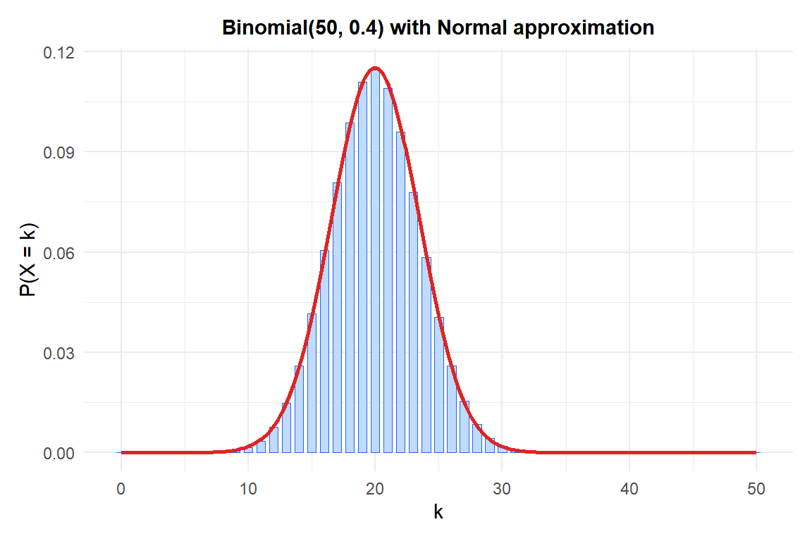
Figure 1: For n=50 and p=0.4 the normal approximation (red curve) fits the binomial PMF closely
💡 Relationship with other distributions
- Bernoulli: \(\text{Binomial}(1, p) = \text{Bernoulli}(p)\).
- Poisson approximation: when \(n\) is large and \(p\) is small, \(\text{Binomial}(n, p) \approx \text{Poisson}(\lambda = np)\).
- Normal approximation: when \(np \geq 5\) and \(n(1-p) \geq 5\).
- Hypergeometric: use instead of binomial when sampling without replacement from a finite population.

