Bernoulli distribution
The Bernoulli distribution models a single trial with exactly two possible outcomes: success (1) with probability \(p\), and failure (0) with probability \(1-p\). It is the simplest discrete distribution and the building block of the binomial distribution.
Definition
A random variable \(X\) follows a Bernoulli distribution with parameter \(p \in [0, 1]\), written \(X \sim \text{Bernoulli}(p)\), if:
\[P(X = x) = p^x (1-p)^{1-x} \quad \text{for } x \in \{0, 1\}\]
Which is equivalent to:
\[P(X = 1) = p \quad \text{(success)}, \qquad P(X = 0) = 1 - p \quad \text{(failure)}\]
The parameter \(p\) is the probability of success. Everything else about the distribution follows from this single number.
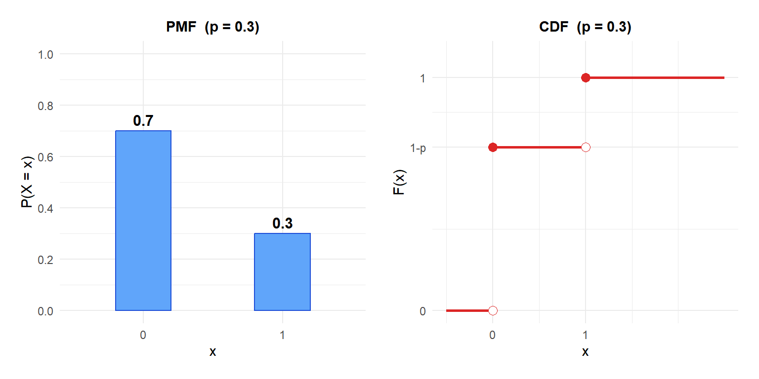
Probability Mass Function and CDF
The PMF assigns probability \(p\) to outcome 1 and \(1-p\) to outcome 0. The CDF is:
\[F(x) = \begin{cases} 0 & \text{if } x < 0 \\ 1-p & \text{if } 0 \leq x < 1 \\ 1 & \text{if } x \geq 1 \end{cases}\]
Properties
For \(X \sim \text{Bernoulli}(p)\):
- Expected Value (Mean)
\[E(X) = p\]
- Variance
\[\text{Var}(X) = p(1-p)\]
Variance is maximized at \(p = 0.5\) (value of \(0.25\)) and equals zero when \(p = 0\) or \(p = 1\) (degenerate cases with no randomness).
- Skewness
\[\text{Skewness} = \frac{1 - 2p}{\sqrt{p(1-p)}}\]
The distribution is symmetric only when \(p = 0.5\). For \(p < 0.5\) it is right-skewed; for \(p > 0.5\) it is left-skewed.
- Kurtosis
\[g_2 = \frac{1 - 6p(1-p)}{p(1-p)}\]
For \(p = 0.5\): \(g_2 = (1 - 1.5)/0.25 = -2\), strongly platykurtic.
- Quantile Function
\[Q(u) = \begin{cases} 0 & \text{if } u \leq 1 - p \\ 1 & \text{if } u > 1 - p \end{cases}\]
Example: product quality control
A factory produces circuit boards with a 15% defect rate. Each board is either defective (success = 1, \(p = 0.15\)) or non-defective (failure = 0, \(1-p = 0.85\)). Let \(X \sim \text{Bernoulli}(0.15)\).
- \(P(X = 1) = 0.15\): probability a randomly selected board is defective.
- \(P(X = 0) = 0.85\): probability it passes inspection.
- \(E(X) = 0.15\): on average, 15% of boards are defective.
- \(\text{Var}(X) = 0.15 \times 0.85 = 0.1275\).
If 200 boards are inspected independently, the total number of defective boards follows a \(\text{Binomial}(200, 0.15)\) distribution, which is a sum of 200 independent Bernoulli(0.15) variables.
- Email spam filter: each incoming email is spam (1) or not (0). If 30% of emails are spam, \(X \sim \text{Bernoulli}(0.3)\).
- Clinical trial: a patient responds to treatment (1) or not (0). If response rate is 60%, \(X \sim \text{Bernoulli}(0.6)\).
- Free throw: a basketball player makes (1) or misses (0) a shot with probability equal to their career average.
⚠️ Do not confuse the parameter p with a p-value
In the Bernoulli distribution, (p) is the probability of success, a fixed characteristic of the process being modeled. A p-value in hypothesis testing is a completely different concept: it is the probability of observing results at least as extreme as the data, assuming the null hypothesis is true. The shared notation causes confusion, especially in introductory courses.
Relationship with the binomial distribution
The Bernoulli distribution is the special case of the binomial distribution with \(n = 1\):
\[\text{Binomial}(1, p) = \text{Bernoulli}(p)\]
More importantly, if \(X_1, X_2, \ldots, X_n\) are independent \(\text{Bernoulli}(p)\) variables, their sum:
\[S = X_1 + X_2 + \cdots + X_n \sim \text{Binomial}(n, p)\]
This is why the Bernoulli distribution is called the building block of the binomial: every binomial count is a sum of independent Bernoulli trials.
💡 When to use the Bernoulli distribution

