Standard deviation and variance in statistics
Variance and standard deviation measure how spread out the values in a dataset are around the mean. They are the most widely used measures of dispersion in statistics, and understanding their differences, including when to divide by \(n\) or \(n-1\), is essential.
Definitions
Variance
Variance measures the average squared distance of each observation from the mean. Squaring the differences serves two purposes: it makes all values positive, and it penalizes large deviations more heavily than small ones.
There are two versions depending on whether you are working with a full population or a sample.
Population variance (when you have data for the entire population):
\[ \sigma^2 = \frac{1}{n} \sum_{i=1}^{n} (x_i - \bar{x})^2 \]
Sample variance (when you are working with a sample and want to estimate the population variance):
\[ s^2 = \frac{1}{n-1} \sum_{i=1}^{n} (x_i - \bar{x})^2 \]
⚠️ Population variance vs. sample variance: the n-1 correction
Dividing by (n-1) instead of (n) in the sample formula is called Bessel’s correction. The reason: when you compute the mean from a sample, you are already using the data to estimate one parameter. This leaves only (n-1) independent pieces of information. Dividing by (n) systematically underestimates the true population variance. Dividing by (n-1) corrects for this bias.
In practice: if your data is the full population, use \(n\). If your data is a sample (which is almost always the case), use \(n-1\). Most software, including R’s var() function, uses \(n-1\) by default.
Standard deviation
Standard deviation is the square root of the variance. The key advantage over variance is that it is expressed in the same units as the original data, making it directly interpretable.
Population standard deviation:
\[ \sigma = \sqrt{\frac{1}{n} \sum_{i=1}^{n} (x_i - \bar{x})^2} \]
Sample standard deviation:
\[ s = \sqrt{\frac{1}{n-1} \sum_{i=1}^{n} (x_i - \bar{x})^2} \]
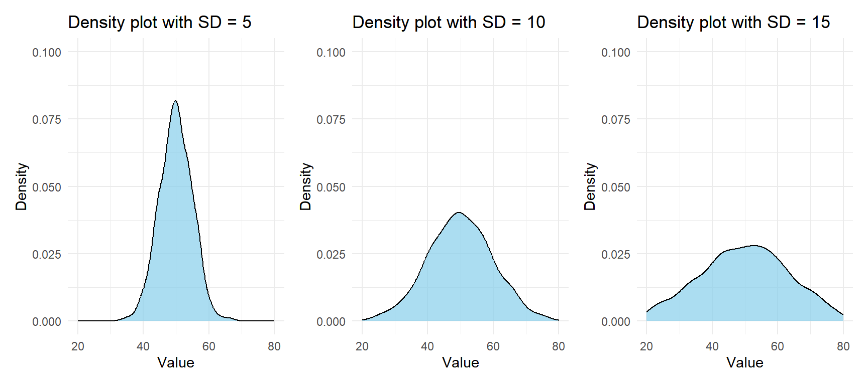
Figure 1: Same mean, different standard deviations: larger SD means a wider, flatter distribution
Properties
- Non-negative: both variance and standard deviation are always \(\geq 0\). They equal zero only when all values are identical.
- Same units: standard deviation is in the same units as the data. Variance is in squared units, which is why standard deviation is usually preferred for interpretation.
- Sensitive to outliers: both measures are influenced by extreme values, since deviations are squared. One outlier can inflate the variance substantially.
- Linear transformation: if \(Y = aX + b\), then \(\sigma_Y = |a| \cdot \sigma_X\) and \(\sigma_Y^2 = a^2 \cdot \sigma_X^2\). Adding a constant does not change the dispersion; multiplying scales it.
⚠️ Variance and standard deviation are not interchangeable
A common exam mistake is using variance and standard deviation as if they measure the same thing on the same scale. If the standard deviation of exam scores is 8 points, the variance is 64 points². Reporting a variance of 64 as if it were “64 points of spread” is wrong: it is 64 squared points. Always report standard deviation when you need an interpretable measure of spread in the original units.
Examples
Example 1: step-by-step calculation
A quality control team measures the weight (in grams) of 5 items from a production batch: \(85, 90, 88, 92, 78\).
Step 1: calculate the mean.
\[\bar{x} = \frac{85 + 90 + 88 + 92 + 78}{5} = 86.6 \text{ g}\]
Step 2: calculate the squared deviations from the mean.
| \(x_i\) | \(x_i - \bar{x}\) | \((x_i - \bar{x})^2\) |
|---|---|---|
| 85 | \(-1.6\) | \(2.56\) |
| 90 | \(3.4\) | \(11.56\) |
| 88 | \(1.4\) | \(1.96\) |
| 92 | \(5.4\) | \(29.16\) |
| 78 | \(-8.6\) | \(73.96\) |
| Sum | \(119.2\) |
Step 3: calculate variance and standard deviation.
Since this is a sample (not the full production batch), we use \(n - 1 = 4\):
\[s^2 = \frac{119.2}{4} = 29.8 \text{ g}^2\]
\[s = \sqrt{29.8} \approx 5.46 \text{ g}\]
The typical item deviates about 5.5 grams from the mean weight.
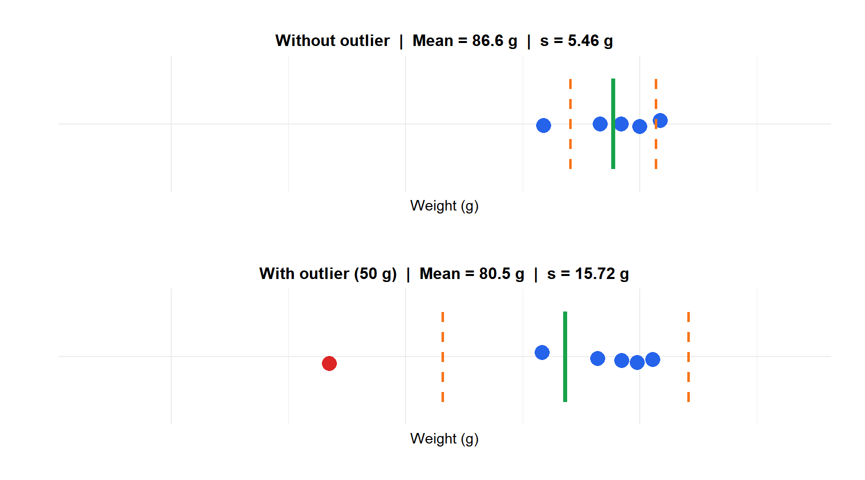
Example 2: the effect of an outlier
Now suppose one defective item slips through with a weight of 50 g. The new dataset is: \(85, 90, 88, 92, 78, 50\).
\[\bar{x} = \frac{85 + 90 + 88 + 92 + 78 + 50}{6} = 80.5 \text{ g}\]
\[s^2 = \frac{(85-80.5)^2 + (90-80.5)^2 + (88-80.5)^2 + (92-80.5)^2 + (78-80.5)^2 + (50-80.5)^2}{5} = \frac{1215.5}{5} = 243.1 \text{ g}^2\]
\[s = \sqrt{243.1} \approx 15.59 \text{ g}\]
One defective item tripled the standard deviation, from 5.46 g to 15.59 g. This is why standard deviation is sensitive to outliers: the squared term amplifies extreme deviations.
💡 When to use standard deviation vs. other measures of dispersion

