Cramér's V
Pearson’s chi-squared test tells you whether an association between two categorical variables is statistically significant. Cramér’s V tells you how strong that association is. You need both.
Definition
Cramér’s V is a measure of the strength of association between two categorical variables. It is derived from the chi-squared statistic and normalized so that it always falls between 0 and 1, regardless of the size of the contingency table:
\[ V = \sqrt{\frac{\chi^2}{n \cdot (\min(r, c) - 1)}} \]
where \(\chi^2\) is the Pearson chi-squared statistic, \(n\) is the total number of observations, \(r\) is the number of rows, and \(c\) is the number of columns in the contingency table.
- \(V = 0\): no association between the variables.
- \(V = 1\): perfect association (knowing one variable completely determines the other).
The denominator \(\min(r, c) - 1\) scales the statistic appropriately for tables of different sizes, which is why Cramér’s V is preferred over simpler measures when the table has more than two categories in either dimension.
Interpretation
Cohen (1988) proposed benchmarks for interpreting Cramér’s V that depend on the degrees of freedom \(df = \min(r,c) - 1\):
| \(df\) | Small | Medium | Large |
|---|---|---|---|
| 1 | 0.10 | 0.30 | 0.50 |
| 2 | 0.07 | 0.21 | 0.35 |
| 3 | 0.06 | 0.17 | 0.29 |
| 4 | 0.05 | 0.15 | 0.25 |
These thresholds matter because a \(V = 0.25\) in a 2×2 table is a medium-to-large effect, while the same value in a 5×5 table is a large effect. Using a single universal threshold for all table sizes is incorrect.
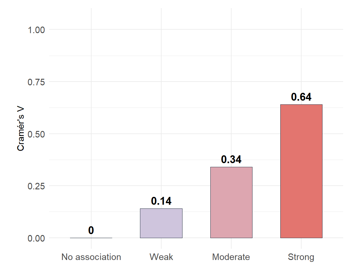
Figure 1: Cramér’s V for simulated contingency tables: from near-zero association (blue) to strong association (red)
⚠️ A significant chi-squared test does not mean a strong association
With large samples, even a tiny real-world association produces a highly significant chi-squared statistic. A study with (n = 10{,}000) can give (p < 0.001) with (V = 0.05), which is a negligible effect. Always compute Cramér’s V alongside the chi-squared test, and always report both the p-value and the effect size.
Step-by-step example
Using the smoking and lung cancer data from the chi-squared post:
| Lung Cancer: Yes | Lung Cancer: No | Total | |
|---|---|---|---|
| Smoker | 70 | 30 | 100 |
| Non-smoker | 20 | 80 | 100 |
| Total | 90 | 110 | 200 |
From the previous calculation, \(\chi^2 = 50.50\), \(n = 200\), \(r = 2\), \(c = 2\).
\[V = \sqrt{\frac{50.50}{200 \cdot (\min(2,2) - 1)}} = \sqrt{\frac{50.50}{200 \cdot 1}} = \sqrt{0.2525} \approx 0.502\]
For a 2×2 table (\(df = 1\)), Cohen’s benchmarks give: small = 0.10, medium = 0.30, large = 0.50. A value of \(V \approx 0.50\) indicates a large association between smoking status and lung cancer in this sample.
Example 2: education level and voting preference
A survey of 300 voters records education level (3 categories) and preferred political party (4 categories). After building the contingency table, the chi-squared statistic is \(\chi^2 = 24.7\).
\[V = \sqrt{\frac{24.7}{300 \cdot (\min(3,4) - 1)}} = \sqrt{\frac{24.7}{300 \cdot 2}} = \sqrt{\frac{24.7}{600}} \approx 0.203\]
For a 3×4 table (\(df = \min(3,4) - 1 = 2\)), Cohen’s benchmarks: small = 0.07, medium = 0.21, large = 0.35. A value of \(V \approx 0.20\) is close to a medium effect, suggesting a moderate association between education and voting preference.
Phi coefficient vs Cramér’s V
The phi coefficient (\(\phi\)) is the special case of Cramér’s V for 2×2 tables:
\[\phi = \sqrt{\frac{\chi^2}{n}}\]
For 2×2 tables, \(\min(r,c) - 1 = 1\), so \(\phi = V\). For tables larger than 2×2, phi is no longer bounded by 1 and loses its interpretability. Cramér’s V generalizes phi correctly to any table size.
💡 Which measure to use
⚠️ Cramér's V is biased with small samples
For small samples ((n < 100)) or sparse tables, Cramér’s V tends to overestimate the true association in the population. A bias-corrected version proposed by Bergsma (2013) is sometimes used in these situations. If your sample is small, check whether your software offers the corrected version before reporting (V).

