Covariance in statistics
Covariance measures whether two variables tend to move in the same direction or in opposite directions. It is the foundation of correlation, regression, and portfolio theory in finance.
Definition
When two variables are measured on the same individuals, covariance tells you whether they tend to increase together (positive covariance), move in opposite directions (negative covariance), or have no consistent linear pattern (zero covariance).
As with variance, there are two versions depending on whether you have a full population or a sample.
Population covariance:
\[ \sigma_{XY} = \frac{1}{n} \sum_{i=1}^{n} (x_i - \bar{x})(y_i - \bar{y}) \]
Sample covariance (used in practice when working with a sample):
\[ s_{XY} = \frac{1}{n-1} \sum_{i=1}^{n} (x_i - \bar{x})(y_i - \bar{y}) \]
The \(n-1\) correction in the sample formula serves the same purpose as in the sample variance: it corrects for the fact that the sample means are themselves estimates, leaving only \(n-1\) independent pieces of information.
Interpretation
The sign of the covariance tells you the direction of the relationship:
- Positive covariance (\(s_{XY} > 0\)): when \(X\) is above its mean, \(Y\) tends to be above its mean too. The variables move together.
- Negative covariance (\(s_{XY} < 0\)): when \(X\) is above its mean, \(Y\) tends to be below its mean. The variables move in opposite directions.
- Zero covariance (\(s_{XY} \approx 0\)): no consistent linear relationship between \(X\) and \(Y\).
The magnitude of covariance is harder to interpret because it depends on the units of both variables. This is the key limitation of covariance compared to correlation.
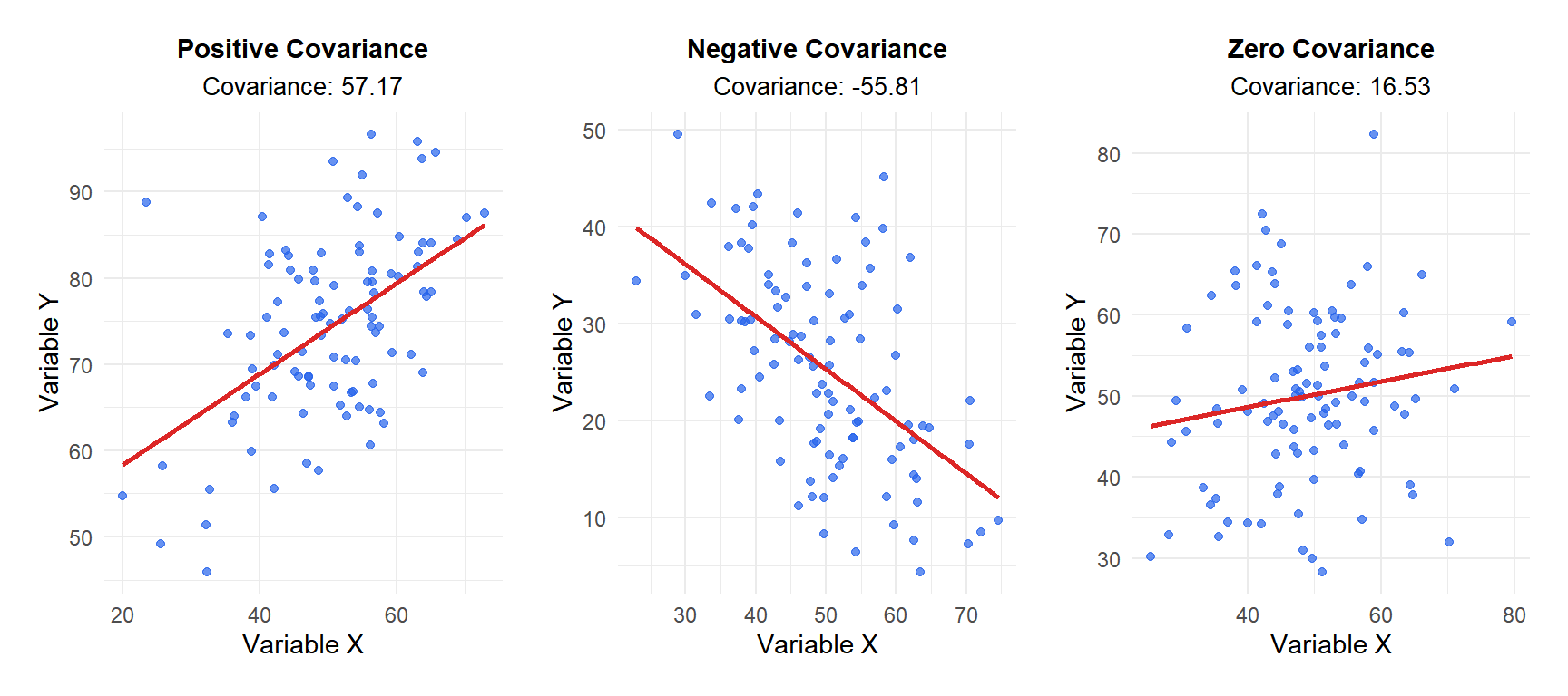
Figure 1: The sign of the covariance indicates the direction of the linear relationship between two variables
⚠️ Zero covariance does not mean independence
Covariance measures linear association only. Two variables can have zero covariance and still be strongly related in a non-linear way. For example, if (Y = X^2) and (X) is symmetric around zero, the covariance between (X) and (Y) is zero, but (Y) is completely determined by (X). Always check a scatter plot alongside the covariance value.
Step-by-step example
A coach records the weekly training hours and race times (in minutes) of 5 athletes:
| Athlete | Hours trained (\(X\)) | Race time (\(Y\)) |
|---|---|---|
| 1 | 5 | 52 |
| 2 | 8 | 46 |
| 3 | 10 | 43 |
| 4 | 12 | 40 |
| 5 | 15 | 35 |
Step 1: calculate the means.
\[\bar{x} = \frac{5+8+10+12+15}{5} = 10, \quad \bar{y} = \frac{52+46+43+40+35}{5} = 43.2\]
Step 2: calculate the deviations and their products.
| \(x_i\) | \(y_i\) | \(x_i - \bar{x}\) | \(y_i - \bar{y}\) | \((x_i-\bar{x})(y_i-\bar{y})\) |
|---|---|---|---|---|
| 5 | 52 | \(-5\) | \(8.8\) | \(-44.0\) |
| 8 | 46 | \(-2\) | \(2.8\) | \(-5.6\) |
| 10 | 43 | \(0\) | \(-0.2\) | \(0.0\) |
| 12 | 40 | \(2\) | \(-3.2\) | \(-6.4\) |
| 15 | 35 | \(5\) | \(-8.2\) | \(-41.0\) |
| Sum | \(-97.0\) |
Step 3: apply the sample covariance formula.
\[s_{XY} = \frac{-97.0}{5-1} = -24.25\]
The covariance is negative: athletes who train more hours tend to have lower (faster) race times. More training is associated with better performance.
The covariance of (-24.25) tells us the direction (negative: more training, faster times) but not the strength of the relationship in any standardized sense. If we had measured race time in seconds instead of minutes, the covariance would be (-24.25 \times 60 = -1455), even though the relationship is identical. This is why correlation is preferred when you want to compare the strength of associations.
The units problem
Covariance is expressed in the product of the units of both variables. If \(X\) is in hours and \(Y\) is in minutes, covariance is in hour·minutes. This makes it:
- Hard to interpret in absolute terms.
- Impossible to compare across different pairs of variables.
- Sensitive to rescaling: multiplying \(X\) by a constant \(a\) and \(Y\) by a constant \(b\) multiplies the covariance by \(a \times b\).
⚠️ Never compare covariances from different datasets directly
A covariance of 500 between height and weight in one study and a covariance of 50 in another does not mean the relationship is ten times stronger in the first. The difference could be entirely due to different units, different scales, or different sample variability. Use correlation for comparisons.
Relationship with correlation
Correlation is covariance divided by the product of the standard deviations of both variables:
\[r_{XY} = \frac{s_{XY}}{s_X \cdot s_Y}\]
This standardization removes the units and constrains the result to \([-1, 1]\), making it directly interpretable and comparable across datasets. In the athletes example:
\[s_X = \sqrt{\frac{(-5)^2+(-2)^2+0^2+2^2+5^2}{4}} = \sqrt{13.5} \approx 3.67 \text{ hours}\]
\[s_Y = \sqrt{\frac{8.8^2+2.8^2+0.2^2+3.2^2+8.2^2}{4}} = \sqrt{43.7} \approx 6.61 \text{ min}\]
\[r_{XY} = \frac{-24.25}{3.67 \times 6.61} \approx -1.00\]
A correlation of \(-1\) indicates a perfect negative linear relationship: in this small dataset, training hours and race time follow an almost perfectly linear pattern.
💡 When to use covariance vs correlation

