Coefficient of skewness in statistics
Skewness measures the asymmetry of a distribution. Knowing whether your data is skewed, and in which direction, affects which summary statistics make sense, which tests are valid, and how to interpret results.
What is skewness?
Most real datasets are not perfectly symmetric. Income distributions have a long right tail (a few people earn vastly more than the rest). Exam scores in a hard test pile up near the bottom. Skewness quantifies this asymmetry.
The most common formula, used by most statistical software, is the adjusted Fisher-Pearson coefficient:
\[ g = \frac{n}{(n-1)(n-2)} \sum_{i=1}^{n} \left(\frac{x_i - \bar{x}}{s}\right)^3 \]
where \(n\) is the sample size, \(\bar{x}\) is the mean, and \(s\) is the sample standard deviation.
The cubic power is what gives skewness its directional sensitivity: positive deviations raised to the third power stay positive, negative deviations stay negative, and large deviations dominate because of the exponent.
Types of skewness
Positive skewness (right-skewed)
When \(g > 0\), the right tail is longer. Most values cluster on the left, with a few high values stretching the distribution to the right. The mean is pulled toward the tail, so:
\[\text{Mode} < \text{Median} < \text{Mean}\]
Real examples: household income, house prices, number of social media followers, insurance claims.
Negative skewness (left-skewed)
When \(g < 0\), the left tail is longer. Most values cluster on the right, with a few low values pulling the distribution to the left:
\[\text{Mean} < \text{Median} < \text{Mode}\]
Real examples: age at retirement, scores on an easy exam, time until failure of high-quality components.
Zero skewness (symmetric)
When \(g \approx 0\), the distribution is symmetric and mean, median and mode coincide. The normal distribution has zero skewness by definition.
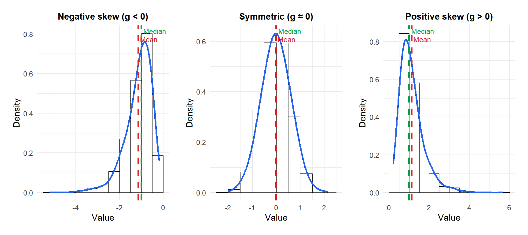
Figure 1: Mean, median and mode shift relative to each other depending on the direction of skewness
⚠️ Skewness shifts the mean away from the center
In a skewed distribution the mean is no longer a good summary of the “typical” value. In a right-skewed income distribution, the mean salary is higher than what most people actually earn, because a few very high earners pull it up. The median is a better measure of central tendency when skewness is present.
How to interpret the coefficient
There is no universal threshold, but common guidelines are:
| Value of \(g\) | Interpretation |
|---|---|
| \(g < -1\) or \(g > 1\) | Highly skewed |
| \(-1 \leq g \leq -0.5\) or \(0.5 \leq g \leq 1\) | Moderately skewed |
| \(-0.5 < g < 0.5\) | Approximately symmetric |
These are rules of thumb, not hard cutoffs. Always look at the histogram alongside the coefficient.
💡 Always plot before interpreting
Step-by-step example
Consider the following dataset, representing the number of customer complaints received per day over 7 days:
\[x = (3, 4, 5, 6, 8, 12, 20)\]
Step 1: calculate the mean.
\[\bar{x} = \frac{3 + 4 + 5 + 6 + 8 + 12 + 20}{7} = 8.29\]
Step 2: calculate the sample standard deviation.
\[s = \sqrt{\frac{\sum_{i=1}^{7}(x_i - 8.29)^2}{6}} \approx 5.96\]
Step 3: calculate the standardized deviations cubed.
| \(x_i\) | \(x_i - \bar{x}\) | \(\left(\frac{x_i - \bar{x}}{s}\right)^3\) |
|---|---|---|
| 3 | \(-5.29\) | \(-0.703\) |
| 4 | \(-4.29\) | \(-0.375\) |
| 5 | \(-3.29\) | \(-0.169\) |
| 6 | \(-2.29\) | \(-0.057\) |
| 8 | \(-0.29\) | \(-0.000\) |
| 12 | \(3.71\) | \(0.271\) |
| 20 | \(11.71\) | \(8.537\) |
| Sum | \(7.504\) |
Step 4: apply the formula.
\[g = \frac{7}{(7-1)(7-2)} \times 7.504 = \frac{7}{30} \times 7.504 \approx 1.75\]
The distribution is highly right-skewed. One day with 20 complaints is pulling the mean up and creating a long right tail. The median (6 complaints) is a more representative summary than the mean (8.29).
Where skewness matters
- Finance: return distributions are rarely symmetric. Positive skewness means occasional large gains; negative skewness means occasional large losses. Many risk models assume normality, which is wrong when skewness is significant.
- Income and wealth: almost always right-skewed. Reporting the mean income of a country overstates what a typical citizen earns.
- Quality control: a skewed defect distribution suggests the process has a directional problem, not just random noise.
- Choosing statistical tests: many parametric tests assume approximate normality. High skewness is a signal to consider non-parametric alternatives or data transformations.
⚠️ Do not assume normality without checking skewness
A common mistake in applied statistics is running a t-test or ANOVA without verifying that the data is approximately symmetric. If skewness is high (say, (|g| > 1)), the p-values from these tests may be unreliable, especially with small samples. Check skewness (and kurtosis) before applying normality-dependent methods.
💡 What to do when data is highly skewed

