What is bootstrap?
The bootstrap, introduced by Bradley Efron in 1979, is a resampling method that estimates the sampling distribution of any statistic by repeatedly drawing samples with replacement from the original data. It requires no assumptions about the population distribution and works for statistics whose theoretical distribution is intractable.
The core idea
Classical inference derives the sampling distribution of \(\hat{\theta}\) from assumptions about the population (e.g., normality). The bootstrap inverts this logic: it uses the data itself as a proxy for the population and simulates the sampling process by resampling from the observed data.
The reasoning: if the sample is a good representation of the population, then samples drawn from the sample with replacement behave like samples drawn from the population. The distribution of \(\hat{\theta}^*\) across many bootstrap samples approximates the true sampling distribution of \(\hat{\theta}\).
The bootstrap principle:
\[\text{Population} \xrightarrow{\text{sample}} \text{Sample} \xrightarrow{\text{resample with replacement}} \text{Bootstrap samples}\]
\[\text{True distribution of } \hat{\theta} \approx \text{Bootstrap distribution of } \hat{\theta}^*\]
The algorithm
Given an original sample \(\mathbf{x} = (x_1, x_2, \ldots, x_n)\) and a statistic of interest \(\hat{\theta} = g(\mathbf{x})\):
- Draw a bootstrap sample \(\mathbf{x}^* = (x_1^*, \ldots, x_n^*)\) of size \(n\) by sampling with replacement from \(\mathbf{x}\).
- Compute \(\hat{\theta}^* = g(\mathbf{x}^*)\).
- Repeat steps 1-2 \(B\) times, obtaining \(\hat{\theta}^*_1, \hat{\theta}^*_2, \ldots, \hat{\theta}^*_B\).
- Use the distribution of \(\{\hat{\theta}^*_b\}\) to estimate the sampling distribution of \(\hat{\theta}\).
\(B = 1{,}000\) is a common minimum for standard error estimation; \(B = 10{,}000\) for confidence intervals.
Example: bootstrap distribution of the median
The sampling distribution of the median has no simple closed form for most populations. Bootstrap provides an empirical approximation.
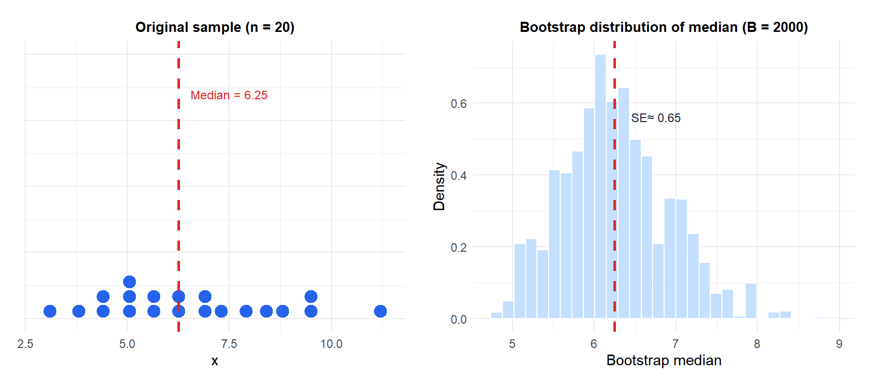
The left panel shows the original sample with its observed median. The right panel shows the distribution of the median across 2,000 bootstrap resamples: approximately normal and centered at the observed median. The standard deviation of this distribution is the bootstrap standard error of the median.
What the bootstrap estimates
The bootstrap distribution of \(\hat{\theta}^*\) centered at \(\hat{\theta}\) approximates the sampling distribution of \(\hat{\theta}\) centered at \(\theta\). From this, we can estimate:
- Standard error: \(\widehat{\text{SE}}_\text{boot} = \text{SD}(\hat{\theta}^*_1, \ldots, \hat{\theta}^*_B)\).
- Bias: \(\widehat{\text{Bias}}_\text{boot} = \bar{\hat{\theta}}^* - \hat{\theta}\), where \(\bar{\hat{\theta}}^*\) is the mean of bootstrap estimates.
- Confidence intervals: percentile, basic, BCa (covered in the bootstrap CI post).
- Sampling distribution shape: useful for detecting skewness or multimodality.
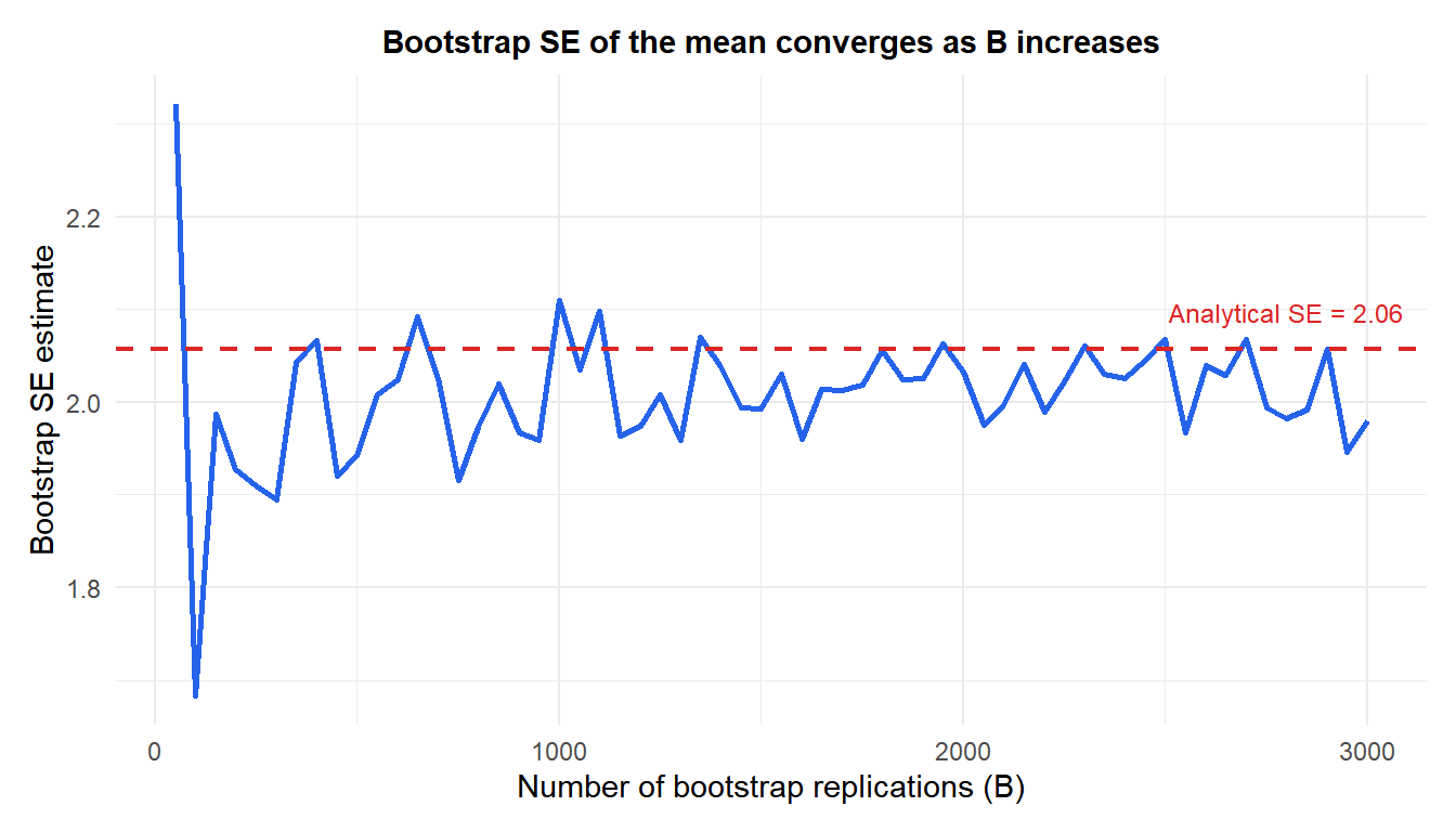
The bootstrap SE converges quickly: by \(B = 500\) it is already close to the analytical value. For confidence intervals, larger \(B\) (typically 2,000–10,000) is recommended for stability in the tails.
Why it works
The bootstrap is justified by the plug-in principle: replace the unknown population distribution \(F\) with the empirical distribution \(\hat{F}_n\) (which places probability \(1/n\) on each observed value). Any functional of \(F\) (mean, variance, quantile) can then be estimated by the corresponding functional of \(\hat{F}_n\).
Resampling with replacement from the original sample is equivalent to sampling from \(\hat{F}_n\). As \(n \to \infty\), \(\hat{F}_n \to F\) (by the Glivenko-Cantelli theorem), so the bootstrap approximation improves with larger samples.
Limitations
⚠️ When the bootstrap fails or performs poorly
The bootstrap is not universally valid. It can fail when:
- Small samples: \(\hat{F}_n\) is a poor approximation of \(F\) with few observations. The smoothed bootstrap (next post) partially addresses this.
- Extreme quantiles: estimating the 99th percentile from \(n = 50\) observations is unreliable even with bootstrap, because the tails of \(\hat{F}_n\) are poorly estimated.
- Dependent data: standard bootstrap assumes i.i.d. observations. For time series, use block bootstrap or circular block bootstrap.
- Non-smooth statistics: the bootstrap can be inconsistent for statistics like the sample maximum or statistics with discontinuities.
When the bootstrap fails, parametric bootstrap (assuming a specific distributional family) is often a better alternative.
💡 How many bootstrap replications?
- Standard error estimation: \(B = 200\)–\(500\) is usually sufficient.
- Percentile confidence intervals: \(B = 1{,}000\)–\(2{,}000\).
- BCa confidence intervals: \(B = 5{,}000\)–\(10{,}000\) for stable results.
- Hypothesis testing p-values: \(B \geq 10{,}000\) for p-values near the significance threshold.
In R: boot::boot(data, statistic, R = 1000). The statistic function must accept the data and an index vector as arguments.

