Smoothed bootstrap
The smoothed bootstrap replaces the discrete empirical distribution \(\hat{F}_n\) with a continuous kernel density estimate \(\hat{f}_h\) before resampling. Instead of drawing from the original data points, it draws from a smoothed version of the data. This reduces the discreteness bias of the uniform bootstrap, particularly for small samples and statistics that depend on the continuity of the distribution.
Motivation: the discreteness problem
The uniform (naive) bootstrap resamples from \(\hat{F}_n\), which places probability mass \(1/n\) on each observed value. For continuous data, this is a discrete approximation of a continuous distribution. The consequence: the bootstrap distribution is also discrete, which can lead to:
- Underestimation of variability for statistics sensitive to the distribution’s shape (quantiles, densities).
- Repeated identical values in resamples, which can distort estimates of range or extremes.
- Rough bootstrap distributions with spikes at observed values.
The smoothed bootstrap spreads each observed point into a small continuous region, producing a smoother and more realistic approximation of the population.
Algorithm
Each smoothed bootstrap observation is generated as:
\[x_i^* = x_{j} + h \cdot \varepsilon_i, \qquad j \sim \text{Uniform}\{1, \ldots, n\}, \quad \varepsilon_i \sim K\]
where \(K\) is a kernel function (commonly \(N(0,1)\)) and \(h > 0\) is the bandwidth. This is equivalent to sampling from the kernel density estimate:
\[\hat{f}_h(x) = \frac{1}{nh} \sum_{i=1}^n K\!\left(\frac{x - x_i}{h}\right)\]
The smoothed bootstrap replaces \(\hat{F}_n\) (empirical distribution) with \(\hat{F}_h\) (kernel CDF). When \(h \to 0\), it reduces to the uniform bootstrap. When \(h \to \infty\), it over-smooths and loses information.
Choosing the bandwidth
The bandwidth \(h\) controls the trade-off between smoothness and fidelity to the data:
- Too small (\(h \to 0\)): reduces to uniform bootstrap. No smoothing benefit.
- Too large: artificially inflates variability beyond what the data supports.
A common default is the Silverman rule of thumb for normal kernels:
\[h = 0.9 \cdot \min\!\left(S, \frac{\text{IQR}}{1.34}\right) \cdot n^{-1/5}\]
For bootstrap purposes, the optimal \(h\) is smaller than for density estimation: using \(h_\text{boot} = h_\text{KDE} / \sqrt{2}\) or \(h_\text{boot} = h_\text{KDE} \cdot n^{-1/10}\) is common in practice.
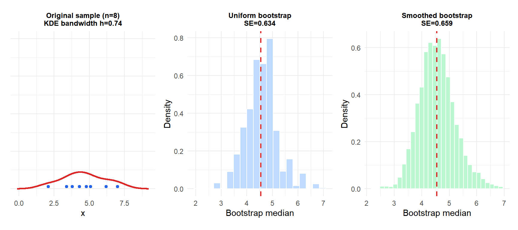
With only 8 observations, the uniform bootstrap distribution of the median (blue) is visibly discrete with spikes at observed values. The smoothed bootstrap (green) produces a continuous, smoother distribution that better represents the underlying uncertainty.
When to use smoothed bootstrap
The smoothed bootstrap is most beneficial when:
- Small samples (\(n < 30\)): the empirical distribution \(\hat{F}_n\) is a poor approximation of \(F\).
- Density or quantile estimation: statistics that depend on the local density of the distribution are sensitive to discreteness.
- Continuous underlying distribution: if the data come from a continuous population, smoothing recovers this continuity.
- Reducing discreteness artifacts: when the uniform bootstrap distribution shows visible spikes or discrete steps.
It is less useful or even harmful when:
- The data are truly discrete (count data, ordinal scales): smoothing distorts the natural discreteness.
- The sample is large: the uniform bootstrap already provides a good approximation.
- The bandwidth is poorly chosen: over-smoothing can inflate variability beyond what the data support.
⚠️ Smoothing is not always better
Adding smoothing introduces a new source of error: the choice of bandwidth. If \(h\) is too large, the smoothed bootstrap generates values far from any observed data, artificially widening the bootstrap distribution. For large samples where the uniform bootstrap works well, smoothing adds complexity without benefit.
A practical guideline: use the uniform bootstrap by default. Switch to smoothed when the uniform bootstrap distribution shows visible discrete spikes or when you are estimating a continuous density.
Example: estimating a quantile
The 75th percentile of a continuous distribution is a smooth functional of \(F\), but the sample quantile from a small dataset can be erratic. Smoothed bootstrap gives a more stable estimate.
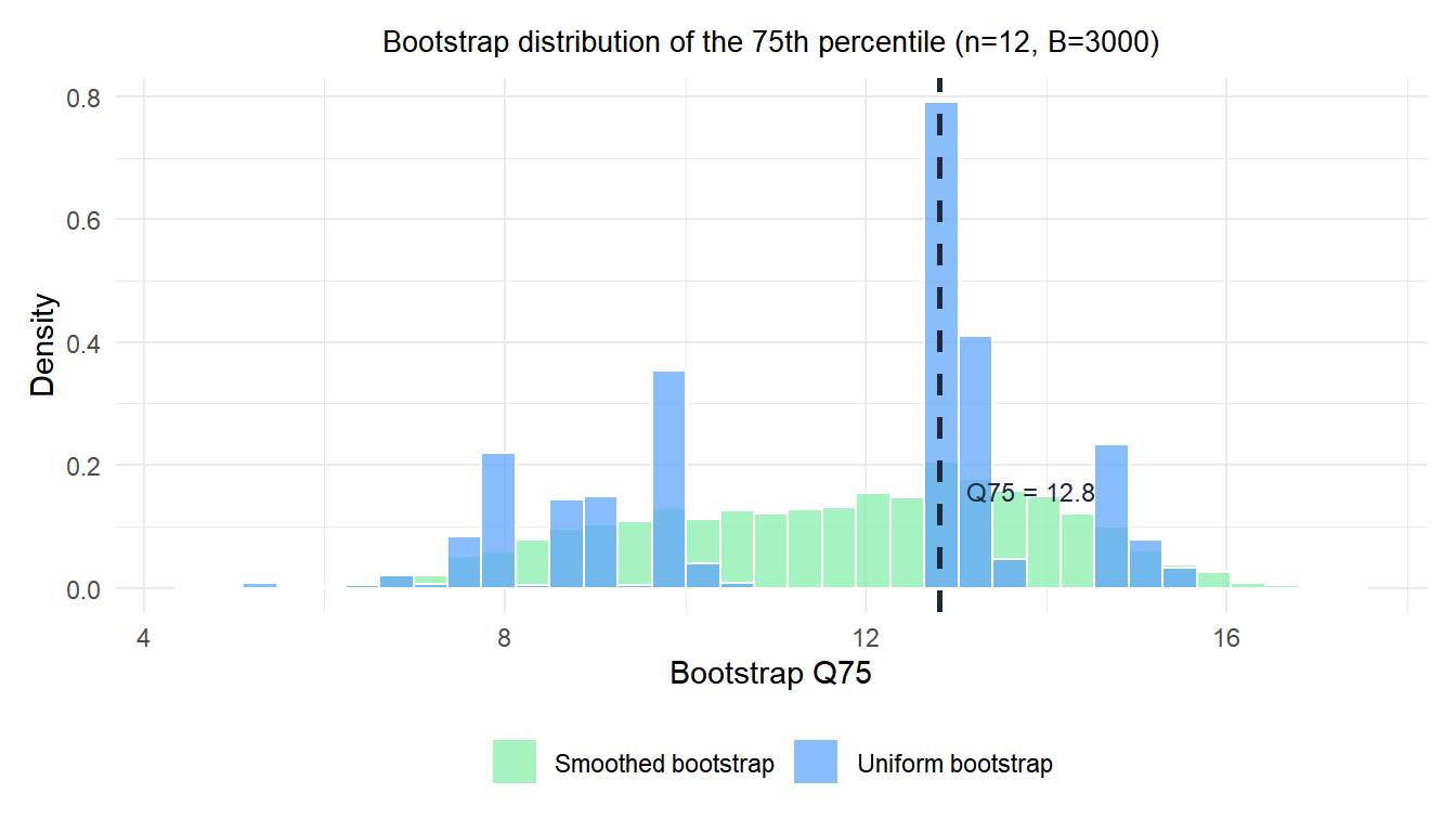
The uniform bootstrap (blue) concentrates mass on the few distinct quantile values possible with \(n=12\). The smoothed bootstrap (green) spreads this mass continuously, providing a more realistic picture of uncertainty in the quantile estimate.
💡 Smoothed bootstrap in R
The boot package does not implement smoothed bootstrap directly, but it is straightforward to implement:
library(boot)

## Define smoothed bootstrap statistic
smooth_boot_stat <- function(data, indices, h) {
  x_resamp <- data[indices] + rnorm(length(indices), 0, h)
  median(x_resamp)  # or any statistic
}

h <- 0.9 * min(sd(x), IQR(x)/1.34) * length(x)^(-0.2) / sqrt(2)
boot(data = x, statistic = smooth_boot_stat, R = 2000, h = h)
