Parametric bootstrap
The parametric bootstrap assumes the data come from a specific distributional family (normal, exponential, Poisson, etc.), fits that distribution to the data, and generates bootstrap samples by simulating from the fitted model. When the model is correctly specified, it is more efficient than the nonparametric bootstrap. When the model is wrong, the results can be misleading.
Algorithm
Given an original sample \(\mathbf{x} = (x_1, \ldots, x_n)\) and an assumed parametric family \(F_\theta\):
- Fit the model: estimate \(\hat{\theta}\) from the data, typically by maximum likelihood.
- Simulate: generate \(B\) bootstrap samples of size \(n\) by drawing from \(F_{\hat{\theta}}\).
- Refit: for each bootstrap sample \(\mathbf{x}^*_b\), re-estimate \(\hat{\theta}^*_b\).
- Summarize: use the distribution of \(\hat{\theta}^*_b\) to estimate the sampling distribution of \(\hat{\theta}\).
\[\mathbf{x}^*_b \sim F_{\hat{\theta}}, \quad b = 1, \ldots, B\]
The key difference from the nonparametric bootstrap: the resamples are drawn from the fitted parametric distribution \(F_{\hat{\theta}}\), not from the empirical distribution \(\hat{F}_n\).
Parametric vs nonparametric bootstrap
| Parametric | Nonparametric (uniform) | |
|---|---|---|
| Resamples from | \(F_{\hat{\theta}}\) (fitted model) | \(\hat{F}_n\) (empirical distribution) |
| Requires distributional assumption | Yes | No |
| Efficiency when model is correct | Higher | Lower |
| Robustness when model is wrong | Poor | Good |
| Suitable for small \(n\) | Yes (if model correct) | Moderate |
| Common use cases | GLMs, survival models, time series | Any statistic, robust analysis |
The parametric bootstrap is more efficient because it uses all the structure imposed by the model: the simulated samples follow the assumed distribution exactly, not the noisy empirical distribution. If the model is correct, this reduces Monte Carlo variance. If the model is wrong, the bootstrap distribution reflects the wrong data-generating process.
Examples
Example 1: exponential distribution
Time between server requests follows an exponential distribution with unknown rate \(\lambda\). From \(n = 25\) observations, \(\hat{\lambda} = 1/\bar{x} = 0.42\) (MLE). Estimate the SE of \(\hat{\lambda}\) and compare parametric vs nonparametric bootstrap.
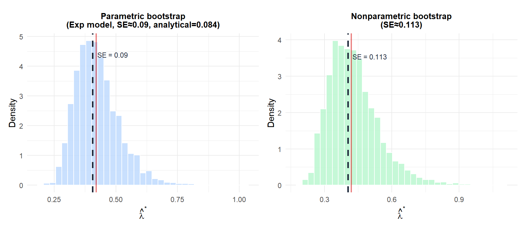
The parametric bootstrap (left) produces a narrower, smoother distribution closer to the analytical SE because it exploits the exponential structure. The nonparametric bootstrap (right) is wider: it makes no distributional assumption and thus has higher Monte Carlo variance. The red line shows the true \(\lambda = 0.42\).
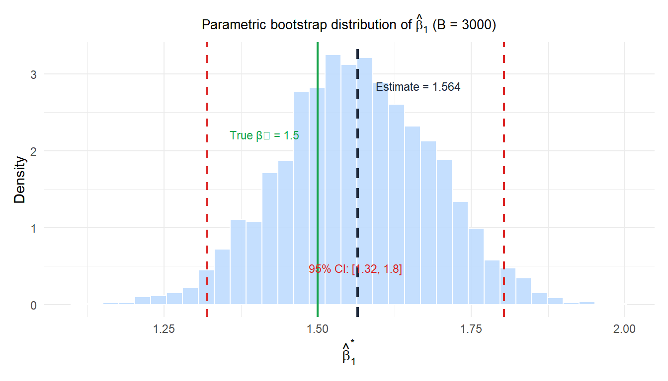
Example 2: parametric bootstrap for a regression model
In regression, the parametric bootstrap fits the model, then simulates new response values from the fitted distribution:
\[y_i^* = \hat{\beta}_0 + \hat{\beta}_1 x_i + \varepsilon_i^*, \qquad \varepsilon_i^* \sim N(0, \hat{\sigma}^2)\]
This generates bootstrap datasets by fixing the design matrix \(X\) and simulating new errors from \(N(0, \hat{\sigma}^2)\). The model is then refit to each bootstrap dataset to obtain \(\hat{\beta}^*_b\).
Model misspecification
⚠️ A wrong model produces wrong bootstrap distributions
The parametric bootstrap is only valid when the assumed distributional family is correct. If you fit a normal distribution to right-skewed data and use parametric bootstrap, the simulated samples will be symmetric while the true data-generating process is asymmetric. The resulting bootstrap SE and CI will be incorrect.
Signs of misspecification to check before using parametric bootstrap:
- Q-Q plot: points should follow the diagonal for the assumed distribution.
- Goodness-of-fit test: Shapiro-Wilk (normal), Kolmogorov-Smirnov (general).
- Residual plots: for regression models, residuals should match the assumed error distribution.
If misspecification is suspected, use the nonparametric or smoothed bootstrap instead.
When to use parametric bootstrap
The parametric bootstrap is the natural choice when:
- A well-justified distributional model exists (exponential for waiting times, Poisson for counts, normal for measurement errors).
- The sample is small and the nonparametric bootstrap has high variance.
- You are working within a modelling framework (GLM, survival model, mixed model) where the parametric structure is part of the inference.
- You need to simulate realistic datasets for power analysis or simulation studies.
💡 Parametric bootstrap in R
# Exponential example
lhat <- 1 / mean(x)
boot_param <- replicate(2000, 1 / mean(rexp(length(x), rate = lhat)))
sd(boot_param)   # bootstrap SE
quantile(boot_param, c(0.025, 0.975))  # 95% CI

# Regression example
fit <- lm(y ~ x)
boot_beta <- replicate(2000, {
  y_star <- fitted(fit) + rnorm(length(y), 0, sigma(fit))
  coef(lm(y_star ~ x))[2]
})
For complex models (GLMs, mixed models), the simulate() function in R generates parametric bootstrap samples from a fitted model object automatically.

