Bootstrap confidence intervals
Bootstrap confidence intervals use the bootstrap distribution of \(\hat{\theta}^*\) to construct a range of plausible values for the true parameter \(\theta\). Four main methods exist, differing in accuracy, assumptions, and computational cost. The BCa interval is the most accurate general-purpose choice.
Setup and notation
From \(B\) bootstrap resamples we have estimates \(\hat{\theta}^*_1, \ldots, \hat{\theta}^*_B\). Let \(\hat{\theta}^*_{(\alpha)}\) denote the \(\alpha\)-quantile of the bootstrap distribution. The observed statistic from the original sample is \(\hat{\theta}\).
- Percentile interval
The simplest method: use the quantiles of the bootstrap distribution directly.
\[\text{CI}_\text{perc} = \left[\hat{\theta}^*_{(\alpha/2)},\; \hat{\theta}^*_{(1-\alpha/2)}\right]\]
Intuition: if the bootstrap distribution is centered at \(\hat{\theta}\) and symmetric, the percentile interval is a valid approximation. Implementation: sort the \(B\) bootstrap estimates and take the \(\lfloor B\alpha/2 \rfloor\) and \(\lceil B(1-\alpha/2) \rceil\) values.
Limitation: the percentile interval ignores bias. If the bootstrap distribution is shifted relative to the true sampling distribution (i.e., \(E[\hat{\theta}^*] \neq \hat{\theta}\) or \(E[\hat{\theta}] \neq \theta\)), the interval has incorrect coverage.
- Basic (reversed) interval
Also called the empirical or pivotal interval. It uses the bootstrap distribution of \(\hat{\theta}^* - \hat{\theta}\) as an approximation for the sampling distribution of \(\hat{\theta} - \theta\):
\[\text{CI}_\text{basic} = \left[2\hat{\theta} - \hat{\theta}^*_{(1-\alpha/2)},\; 2\hat{\theta} - \hat{\theta}^*_{(\alpha/2)}\right]\]
Intuition: reflect the bootstrap distribution around \(\hat{\theta}\). This corrects for bias in the location of the bootstrap distribution but not for skewness. The bounds are “reversed”: the upper bound uses the lower bootstrap quantile and vice versa.
- Studentized (bootstrap-t) interval
The most accurate interval when a standard error estimate is available. It standardizes the bootstrap statistic by its own SE:
\[t_b^* = \frac{\hat{\theta}^*_b - \hat{\theta}}{\widehat{\text{SE}}^*_b}\]
\[\text{CI}_\text{stud} = \left[\hat{\theta} - t^*_{(1-\alpha/2)} \cdot \widehat{\text{SE}},\; \hat{\theta} - t^*_{(\alpha/2)} \cdot \widehat{\text{SE}}\right]\]
where \(\widehat{\text{SE}}^*_b\) is the SE of \(\hat{\theta}^*_b\) estimated from a nested bootstrap within each resample (or analytically if available), and \(\widehat{\text{SE}}\) is the SE from the original sample.
Advantage: accounts for varying SE across bootstrap resamples, achieving second-order accuracy. Disadvantage: requires \(B \times B\) nested bootstrap or an analytical SE formula, making it computationally expensive.
- BCa interval (bias-corrected and accelerated)
The standard recommendation for general use. It adjusts the percentile interval for both bias and skewness using two quantities:
- Bias-correction \(\hat{z}_0\): measures how far the bootstrap distribution is shifted from \(\hat{\theta}\).
- Acceleration \(\hat{a}\): measures how the SE of \(\hat{\theta}\) changes with the true parameter value (estimated via jackknife).
\[\hat{z}_0 = \Phi^{-1}\!\left(\frac{\#\{\hat{\theta}^*_b < \hat{\theta}\}}{B}\right)\]
\[\hat{a} = \frac{\sum_{i=1}^n (\bar{\psi} - \psi_i)^3}{6\left[\sum_{i=1}^n (\bar{\psi} - \psi_i)^2\right]^{3/2}}, \quad \psi_i = \hat{\theta}_{(i)} \text{ (jackknife)}\]
\[\alpha_1 = \Phi\!\left(\hat{z}_0 + \frac{\hat{z}_0 + z_{\alpha/2}}{1 - \hat{a}(\hat{z}_0 + z_{\alpha/2})}\right), \quad \alpha_2 = \Phi\!\left(\hat{z}_0 + \frac{\hat{z}_0 + z_{1-\alpha/2}}{1 - \hat{a}(\hat{z}_0 + z_{1-\alpha/2})}\right)\]
\[\text{CI}_\text{BCa} = \left[\hat{\theta}^*_{(\alpha_1)},\; \hat{\theta}^*_{(\alpha_2)}\right]\]
When \(\hat{z}_0 = 0\) (no bias) and \(\hat{a} = 0\) (no skewness), BCa reduces to the percentile interval. BCa achieves second-order accuracy: its coverage error is \(O(n^{-1})\) vs \(O(n^{-1/2})\) for the percentile interval.
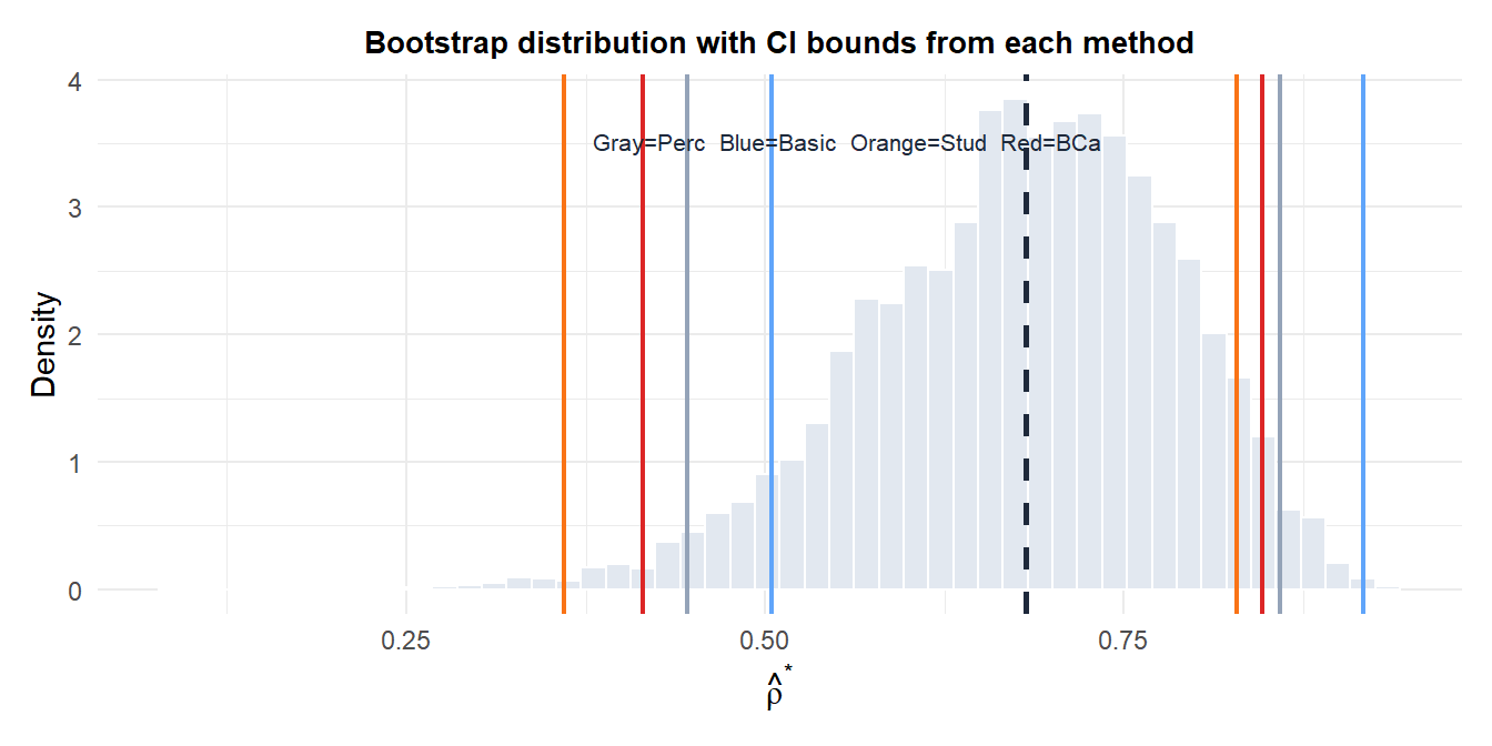
Comparison of the four methods
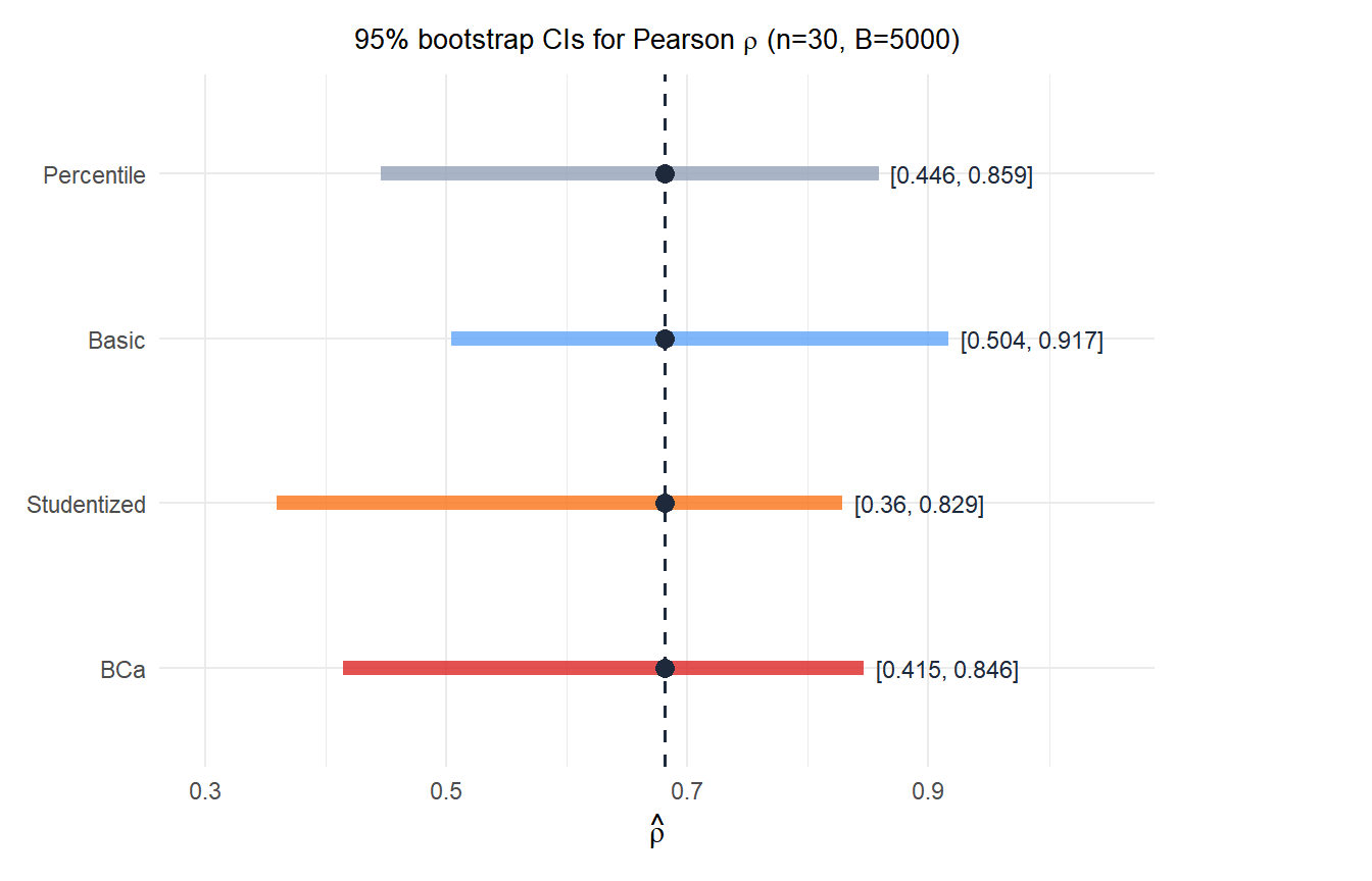
The four intervals differ in location and width because they make different corrections for bias and skewness. For a near-boundary correlation (\(\hat{\rho} \approx 0.8\)), the distribution is left-skewed and BCa produces the most appropriate asymmetric interval.
Which method to use
| Method | Accuracy | Requires | Best for |
|---|---|---|---|
| Percentile | First-order | \(B \geq 1000\) | Quick estimates, symmetric distributions |
| Basic | First-order | \(B \geq 1000\) | Corrects location bias |
| Studentized | Second-order | SE per resample | Pivot-able statistics with available SE |
| BCa | Second-order | \(B \geq 5000\) + jackknife | General purpose, asymmetric distributions |
⚠️ The percentile interval can have poor coverage for skewed or biased statistics
The percentile interval assumes the bootstrap distribution has the same shape as the true sampling distribution. When \(\hat{\theta}\) is biased or its distribution is skewed (common for bounded statistics like correlations, proportions, and variances), the percentile interval has actual coverage below the nominal level.
For a correlation near \(\pm 1\), variances, and other bounded parameters, always prefer BCa over percentile. For the sample mean from a symmetric distribution, all four methods give similar results.
💡 Bootstrap CIs in R with the boot package
library(boot)

stat_fn <- function(data, idx) median(data[idx])
boot_obj <- boot(x, stat_fn, R = 5000)

# All four intervals at once
boot.ci(boot_obj, conf = 0.95,
        type = c("perc", "basic", "stud", "bca"))
For the studentized interval, the statistic function must return a vector c(estimate, variance). For BCa, at least \(B = 2000\) is recommended; \(B = 5000\) for stability in the tails.

